Lesson 12 - Neutron sources
Chapter 4 is concerned with the description of the physical mechanisms that give rise
to neutron, gamma ray, or x-ray sources. The chapter forms a excellent reference for
all sorts of useful information, but we are going to be more selective with the material
we concentrate on. Source description is the first step of any shielding analysis.
In many cases, the particle sources will be known from:
- The problem specification (especially for "made up" problems for method
verification studies or from standardized conservative sources specified by some industry
standard); or
- A previous analysis (especially for reactor shielding studies).
The other cases is the situation where material properties
are specified and the analyst has to deduce the source from this known material.
This is the situation that we will be concentrating on.
Basically, we will be looking at the MAJOR sources of particles that I think you should
be aware of, with an eye toward sensitizing you to look for sources that are likely to
"sneak up" on you if you are not careful. (Our greatest danger is to
underestimate a source because we overlook a complete category.)
The book lists 5 neutron source categories:
- Fission sources
- Photoneutron sources
 sources
- Activation neutrons
- Fusion neutrons
From the reading, you should be able to describe the physical mechanism for each of
these (as I had you do in the Reading Assignment) and work very simple problems that
require basic skills you already have (e.g., atom density determinations for nuclides,
time-dependent buildup and decay, reaction rate determination from fluxes and cross
sections).
In addition, we will be covering more detail about two of these, which are the
mechanisms of spontaneous fission and sources due to reactions.
In addition, as the last section of this lesson, we will briefly
explore the idea of multigroup energy representation.
Spontaneous Fission Sources
The first of the neutron that we will concentrate on is spontaneous fission, which is a
version of fission that occurs without the benefit of an inducing neutron being absorbed.
Several notes:
- Since there is no incoming neutron, the reaction doesn't have the advantage of the
neutron's kinetic and (especially) binding energy to speed up the reaction.
Therefore, the reaction time is slow, with half-lives in years instead of nanoseconds.
- Because there is no incoming neutron, the underlying nucleus must "supply" it.
This is a strange way of saying that the predominant spontaneous
fission nuclides have a mass one greater than the predominant induced
fission nuclides. For example, the primary fissile plutonium isotopes are the odd
isotopes, Pu-235, -237, -239, -241, and -243; the corresponding primary spontaneous
fission nuclides are the even isotopes, Pu-236,-238, -240, -242, and
Pu-244.
- This is a single-nuclide reaction, so it is independent of the chemical or physical form
of the underlying material, but depends only on its mass.
When considering any of these sources, we are concerned with two factors: the yield
(number of particles produced) and the spectrum (energy distribution of
the particles produced).
For spontaneous fission, the yield depends only on the underlying mass; the most
convenient form of data for this is usually something like the last column of Table 4.2.
You should be able to determine spontaneous fission yields with data from this
table.
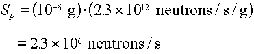
Example: What is the neutron source rate from a 1 microgram point
source of Cf-252?
Answer: From Table 4.2, the spontaneous fission yield of  neutrons/sec/gram.
Therefore the source rate is: neutrons/sec/gram.
Therefore the source rate is:
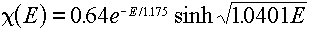
For the spectrum, we generally use the Watt spectrum form given by Equations 4.1 and
4.2 (with data from Table 4.3). Note from Figure 4.1 that all nuclides have a
similar shape, differing primarily in the high-energy "tail". (Note that
the plotted spectra differ by about a factor of 10 at 15 MeV in Figure 4.1.) This
difference can be more significant than the logarithmic y-axis of this figure implies,
since it is these high energy particles that are most likely to penetrate shielding.
Notice, though, the mixed nature of Figure 4.1 . For all isotopes except Cf-252,
the curve is for induced fission; therefore, to use the figure for spontaneous
fission, one has to recognize that the spontaneously fissioning nuclide is the nuclide we
have AFTER the inducing neutron has been absorbed. For example, the curve for
induced Pu-239 fission corresponds to spontaneous Pu-240 fission (since, of course, for a
neutron causing a fission in Pu-239, the nuclide that breaks apart is the compound nucleus
Pu-240).
Sources
The second neutron source mechanism that we will concentrate on is the reaction.
The physical mechanism of this is that an energetic alpha particle (produced by an emitter
nuclide) breaks through the Coulomb barrier of the nucleus of a second nuclide (called the
converter nuclide) and is absorbed. Subsequently, the compound
nucleus emits a neutron.
Several notes:
- The partnership between the emitter and the converter is a Mutt-and-Jeff relationship.
Most alpha emitters tend to be very heavy nuclides. (Below a certain point in
the periodic chart, radioactive nuclides tend to decay with beta emission.). In
contrast, most converter nuclides have to be very light nuclides, since the Coulomb
barrier of a nucleus rises as the charge of the nucleus increases. (See Table 4.6.)
- The Coulomb barrier is usually the minimum energy that the alpha particle must have to
cause an reaction in the converter, but sometimes the threshold energy is the minimum
energy. (In the Table 4.6 data, this only happens for the two Li isotopes.)
- Because of this threshold energy, the alpha particles are only "at risk" of
inducing an reaction from their birth energy to the threshold energy. Of course, if
the alpha particle's energy goes below the threshold energies of all isotopes in the
material, it cannot enter any nucleus and is destined to slow down, collect a couple of
electrons, and go through life as a helium atom.
- Also because of the threshold energy (and the fact that alpha particle ranges go up
faster than E), yields go up faster than E as well. Equation 4.7 gives us the optimum
yield in Be as a function of alpha energy: As you can see, the yield goes up even
faster than E squared.
-
yields are LOW. Note that Table 4.7 gives the number of neutrons per MILLION alpha
particles.
Let's discuss "optimum yield". As mentioned in the book, the highest
yield that can come from a given energy alpha in a given converter material will occur
when the alpha slows down in a medium that is "pure" converter. For
example, the optimum yield of 0.000110 neutrons/alpha for Cm-242/Be corresponds to the
characteristic Cm-242 alphas being released into a material that is 100% Be.
Why does this matter? Well, alpha particles have a limited range. So, if
they are going to interact with Be to produce the neutrons, the yield is going to be
directly proportional to the number of Be nuclei that the alpha comes into contact with
before it slows down below the Be threshold of 2.6 MeV.
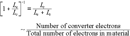
The  part of the book's Equation 4.6 is there to take care of this factor, where the L factors
are stopping powers for the emitter and the converter (Be, in this case). Rather
than get caught up in complicated determinations of these stopping powers -- which was
covered in a part of Chapter 3 that we didn't study (note also that the description of
Equation 4.6 in the text refers you to "Section 3.9", which doesn't exist), we
are going to use the simplified idea that stopping power is approximately proportional to
electron density:
part of the book's Equation 4.6 is there to take care of this factor, where the L factors
are stopping powers for the emitter and the converter (Be, in this case). Rather
than get caught up in complicated determinations of these stopping powers -- which was
covered in a part of Chapter 3 that we didn't study (note also that the description of
Equation 4.6 in the text refers you to "Section 3.9", which doesn't exist), we
are going to use the simplified idea that stopping power is approximately proportional to
electron density:
Example: What would the approximate neutron yield (in
neutrons/alpha) be for  ? ?
Answer: The optimum yield for Am-241/F is given in
Table 4.7 as 4.1 neutrons/million alphas, or 0.0000041= 4.1E-6 neutrons/alpha. Since
this is not a pure F material, we reduce this by the ratio of F electrons to total
electrons:
Since F is element number 9, number of fluorine electrons per molecule is
2 * 9 = 18.
Since Am is element number 95, the total number of electrons in a molecule
is 18 + 95 = 113.
Therefore, the approximate mixture neutron yield would be 4.1E-6*18/113 =
6.5E-7.
Again, once we have the neutron yield (and from a given problem's material
composition, we can easily convert this to a neutron source), we have to consider the
energy distribution of the neutrons that are produced (i.e., the emitted neutron spectrum).
The continuous energy spectra for various emitter-converter combinations are
given in Figure 4.3 in the text.
Multigroup energy representation
Most industry standard computer codes (MCNP being the primary exception)
do not represent energy-dependent data as continuous functions (or distributions), but
instead approximate the continuous data as histograms (i.e., stair-step
functions) which are constant over sub-divisions of the energy range. These energy
subdivisions are refereed to as "energy groups" and are, by
historical convention, numbered sequentially from high to low energies. For example,
if we divide the neutron energy range logarithmically (which is standard for neutron
groups) from 1 keV to 20 MeV with 3 groups per decade, we would get the following
structure:
Note that the highest energy limit (i.e., the top of group 1) is called  .
Also, this is just an example. Usually neutron energy group structures go down to
thermal range, bottoming out at about 0.001 eV (=0.000000001 MeV). .
Also, this is just an example. Usually neutron energy group structures go down to
thermal range, bottoming out at about 0.001 eV (=0.000000001 MeV).
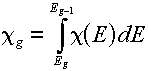
Multigroup representations of distributions
For a distribution,  , (which, you will remember would have "per unit energy"
units), the corresponding group value is found by a simple integration over the energy
range of the group: , (which, you will remember would have "per unit energy"
units), the corresponding group value is found by a simple integration over the energy
range of the group:
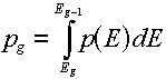
The best examples of when you would do this are the energy spectra (e.g.,
the Watt fission spectrum) described in this lesson. The resulting group value
corresponds to the fraction of produced particles that would be emitted
in the given group.
Note: Be sure that the sum of your group values is 1.0.
If not, you will need to normalize the values by dividing each group value by the
sum of all group values.
For example, if we normalize the Watt spectrum representation of the
Cf-252 fission spectrum (given by Equation 4.2 with Table 4.3 data inserted):
we would get the following values (in the above energy group structure):
Group number, g |
Upper limit of group,  |
 |
| 1 |
20. MeV |
0.00231 |
| 2 |
10. |
0.06579 |
| 3 |
5. |
0.35378 |
| 4 |
2. |
0.28434 |
| 5 |
1. |
0.16783 |
| 6 |
0.5 |
0.09007 |
| 7 |
0.2 |
0.02269 |
| 8 |
0.1 |
0.00845 |
| 9 |
0.05 |
0.00355 |
| 10 |
0.02 |
0.00079 |
| 11 |
0.01 |
0.00028 |
| 12 |
0.005 |
0.00011 |
| 13 |
0.002 |
.00003 |
| 14 |
0.001 = 1 keV |
.00001 |
NOTE: The integrations were done using an S32
Gauss-Legendre quadrature integration. The FORTRAN coding for this is given here, in case you are interested.
You can "eyeball" a spectrum from a spectrum plot by estimating the average
value over the group range and multiplying by the group width.
Example: Verify that the above value for group 3 is reasonable using
Figure 4.1 in the text.
Answer: Group 3 goes from 2 MeV to 5 MeV. The value of the
function falls over the group from about 0.2 (or so) to 0.03. If we take the average
of these as an average value and multiply by the group width, we get 0.115*3 = 0.345 as
our estimate. This compares okay with the 0.354 value in the table.
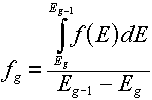
Multigroup representations of functions
Although in this lesson we are only interested in distributions, for completeness it
should be mentioned that for functions of energy (e.g., cross sections) the group value
corresponds to the average value of the function over the energy range, so we have to
divide by the energy width. For example, for a function  , the group
value would be given by the equation: , the group
value would be given by the equation:
|
 NE406
Radiation Protection and Shielding
NE406
Radiation Protection and Shielding