ne.gif (2791 bytes) NE406 Radiation Protection and Shielding

Lesson 7: Interaction coefficients

In this lesson, we take concepts that you have already familiar from your previous study of neutron cross sections and relate them to the slightly different notation that is predominant in describing photon interactions. For this course, we need to be familiar with both nomenclatures. In addition, this lesson describes the scattering interaction coefficients in terms of distributions in energy and direction for the particle after the scattering event.

Interaction coefficient = Macroscopic cross-section

In previous courses, you have learned the concept of the macroscopic cross section, , for a material as the probability of interaction per unit path, with units of . For photons, the traditional symbol for this is ; same idea, same unit.

Other variations that your are used to carry over to the new notation:

= linear absorption coefficient (Not QUITE equivalent, but we will cover the different in a later lesson)
= linear scattering coefficient
gives a collision rate in interactions/cc/sec just like
a given is associated with a particle type and a particular material
is usually dependent on the energy of the particle, which is denoted as .

Note: One notational convention that does not carry over is that we do not use the subscript "t" on for "total". Instead, the "bare" corresponds to the neutron notation of macroscopic total cross section .

is referred to as the linear attenuation coefficient, since it is the coefficient by which a photon population decreases ("attenuates") as it penetrates a material (i.e., ).

Use of mass interaction and attenuation coefficients

One other convention that we will have to get used to is that the photon interaction coefficients themselves are not usually tabulated (i.e., presented in data tables or problem descriptions) as the values we have discussed, but instead as this value divided by the material density, , which has units of and is referred to as the mass interaction (or attenuation) coefficients. (i.e.,The word "linear" is replaced with the word "mass".)

This has been found to be useful for a number of reasons:

Where, as we have seen, the product of flux and linear interaction coefficient, , gives us interaction rate per unit volume, the product of flux and mass interaction coefficient, , gives us interaction rate per unit mass.

As we will see in Chapter 5, the concept of dose, in units of rad, is a measure of energy deposition per unit mass, which fits this unit better..
For photons, is often almost the same AT THE SAME ENERGY for different materials. (Water is the main exception.) As we will see, photon interactions tend to be driven by the presence of electrons. Since materials tend to have similar numbers of electrons/unit mass, this uniformity results.
It really helps when your data is missing an element.

Note: It is somewhat surprising (to me, at least) to compare the data in Tables C.5 on pages 451 and 452. It shows that the mass interaction coefficients for air and water are very similar. (The principal difference is that water has a substantial hydrogen content. Hydrogen delivers more electrons per unit mass than any other element.)

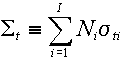
Since it is per unit mass, it applies just as well to elements as to materials. The neutron community uses a microscopic cross section for individual isotopes and builds macroscopic cross sections from them using isotope densities:

wpeB1.gif (1212 bytes)

where I = number of isotopes

= number density of isotope i (nuclei/barn/cm)

= microscopic total cross section of isotope i (barns)

No such juggling of units is needed if we stay on a per mass basis, since:

wpeB5.gif (1599 bytes)

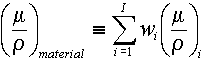
where =mass fraction of isotope i in the material